Introduction
本文为斯坦福大学CS231n课程作业及总结,若有错误,欢迎指正。
所有代码均已上传到GitHub项目 [ cs231n-assignment1 ] ( https://github.com/notplus/cs231n-assignment/tree/master/assignment1 )
Code
1. 通过循环计算Loss和梯度
实现思路: 通过微分公式,计算梯度,只有 margin 中大于0的对梯度有贡献,公式如下:
$L_{i}=\ sum {j \ neq y{i}}\ left [\ max \ left (0, w_{j}^{T} x_{i}-w_{y_{i}}^{T} x_{i}+\ Delta \ right )\ right ]$
$\ nabla {w{y_{i}}} L_{i}=-\ left (\ sum {j \ neq y{i}} \ mathbb {1} \ left (w_{j}^{T} x_{i}-w_{y_{i}}^{T} x_{i}+\ Delta >0\ right )\ right ) x_{i}$
其中 1 是一个示性函数,如果括号中的条件为真,那么函数值为1,如果为假,则函数值为0。
$\ nabla {w{j}} L_{i}=1\ left (w_{j}^{T} x_{i}-w_{y_{i}}^{T} x_{i}+\ Delta >0\ right ) x_{i}$
def   svm_loss_naive ( W ,  X ,  y ,  reg ):
     """
    Structured SVM loss function, naive implementation (with loops).

    Inputs have dimension D, there are C classes, and we operate on minibatches
    of N examples.

    Inputs:
    - W: A numpy array of shape (D, C) containing weights.
    - X: A numpy array of shape (N, D) containing a minibatch of data.
    - y: A numpy array of shape (N,) containing training labels; y[i] = c means
      that X[i] has label c, where 0 <= c < C.
    - reg: (float) regularization strength

    Returns a tuple of:
    - loss as single float
    - gradient with respect to weights W; an array of same shape as W
    """
    dW  =  np. zeros (W.shape)    # initialize the gradient as zero

     # compute the loss and the gradient
    num_classes  =  W.shape[ 1 ]
    num_train  =  X.shape[ 0 ]
    loss  =   0.0
     for  i  in   range (num_train):
        scores  =  X[i]. dot (W)
        correct_class_score  =  scores[y[i]]
         for  j  in   range (num_classes):
             if  j  ==  y[i]:
                 continue
            margin  =  scores[j]  -  correct_class_score  +   1     # note delta = 1
             if  margin  >   0 :
                loss  +=  margin
                dW[:, j]  +=  X[i].T
                dW[:, y[i]]  +=   - X[i].T


     # Right now the loss is a sum over all training examples, but we want it
     # to be an average instead so we divide by num_train.
    loss  /=  num_train

     # Add regularization to the loss.
    loss  +=  reg  *  np. sum (W  *  W)

     #############################################################################
     #  TODO :                                                                     #
     # Compute the gradient of the loss function and store it dW.                #
     # Rather that first computing the loss and then computing the derivative,   #
     # it may be simpler to compute the derivative at the same time that the     #
     # loss is being computed. As a result you may need to modify some of the    #
     # code above to compute the gradient.                                       #
     #############################################################################
     # *****START OF YOUR CODE (DO NOT DELETE/MODIFY THIS LINE)*****

    dW  /=  num_train
    dW  +=  reg  *  W

     # *****END OF YOUR CODE (DO NOT DELETE/MODIFY THIS LINE)*****

     return  loss, dW
2. 实现svm_loss_vectorized 函数
实现思路:
- 主要使用向量化解决,计算loss灵活应用整型访问和广播机制,计算grad灵活应用矩阵乘法,通过构造矩阵乘法免去累加和循环
- 通过
scores[range(num_train), list(y)].reshape(-1,1)生成(N, 1)大小的数组,即按顺序的N个训练样本的正确类别的得分 coeff_mat[margins > 0] = 1coeff_mat[range(num_train), list(y)] = 0
def   svm_loss_vectorized ( W ,  X ,  y ,  reg ):
     """
    Structured SVM loss function, vectorized implementation.

    Inputs and outputs are the same as svm_loss_naive.
    """
    loss  =   0.0
    dW  =  np. zeros (W.shape)  # initialize the gradient as zero

     #############################################################################
     #  TODO :                                                                     #
     # Implement a vectorized version of the structured SVM loss, storing the    #
     # result in loss.                                                           #
     #############################################################################
     # *****START OF YOUR CODE (DO NOT DELETE/MODIFY THIS LINE)*****

    num_train  =  X.shape[ 0 ]
    num_classes  =  W.shape[ 1 ]

    scores  =  X. dot (W)   # (N, C)
    correct_class_scores  =  scores[ range (num_train),  list (y)]. reshape ( - 1 , 1 )  #(N, 1)
    margins  =  np. maximum ( 0 , scores  -  correct_class_scores  + 1 )
    margins[ range (num_train),  list (y)]  =   0

    loss  =  np. sum (margins)
    loss  /=  num_train
    loss  +=  reg  *  np. sum (W  *  W)

     # *****END OF YOUR CODE (DO NOT DELETE/MODIFY THIS LINE)*****

     #############################################################################
     #  TODO :                                                                     #
     # Implement a vectorized version of the gradient for the structured SVM     #
     # loss, storing the result in dW.                                           #
     #                                                                           #
     # Hint: Instead of computing the gradient from scratch, it may be easier    #
     # to reuse some of the intermediate values that you used to compute the     #
     # loss.                                                                     #
     #############################################################################
     # *****START OF YOUR CODE (DO NOT DELETE/MODIFY THIS LINE)*****

     # dw(D,C)  X(N,D)  margins(N,C)
    coeff_mat  =  np. zeros ((num_train, num_classes))
    coeff_mat[margins  >   0 ]  =   1
    coeff_mat[ range (num_train),  list (y)]  =   0
    coeff_mat[ range (num_train),  list (y)]  =   - np. sum (coeff_mat,  axis = 1 )

    dW  =  (X.T). dot (coeff_mat)
    dW  /=  num_train
    dW  +=  reg  *  W

     # *****END OF YOUR CODE (DO NOT DELETE/MODIFY THIS LINE)*****

     return  loss, dW
3. 完成train函数
实现思路:
通过np.random.choice随机选择batchsize大小样本用于计算loss和grad,更新权重
     def   train ( self ,  X ,  y ,  learning_rate = 1e-3 ,  reg = 1e-5 ,  num_iters = 100 ,
               batch_size = 200 ,  verbose = False ):
         """
        Train this linear classifier using stochastic gradient descent.

        Inputs:
        - X: A numpy array of shape (N, D) containing training data; there are N
          training samples each of dimension D.
        - y: A numpy array of shape (N,) containing training labels; y[i] = c
          means that X[i] has label 0 <= c < C for C classes.
        - learning_rate: (float) learning rate for optimization.
        - reg: (float) regularization strength.
        - num_iters: (integer) number of steps to take when optimizing
        - batch_size: (integer) number of training examples to use at each step.
        - verbose: (boolean) If true, print progress during optimization.

        Outputs:
        A list containing the value of the loss function at each training iteration.
        """
        num_train, dim  =  X.shape
        num_classes  =  np. max (y)  +   1   # assume y takes values 0...K-1 where K is number of classes
         if   self .W  is   None :
             # lazily initialize W
             self .W  =   0.001   *  np.random. randn (dim, num_classes)

         # Run stochastic gradient descent to optimize W
        loss_history  =  []
         for  it  in   range (num_iters):
            X_batch  =   None
            y_batch  =   None

             #########################################################################
             #  TODO :                                                                 #
             # Sample batch_size elements from the training data and their           #
             # corresponding labels to use in this round of gradient descent.        #
             # Store the data in X_batch and their corresponding labels in           #
             # y_batch; after sampling X_batch should have shape (batch_size, dim)   #
             # and y_batch should have shape (batch_size,)                           #
             #                                                                       #
             # Hint: Use np.random.choice to generate indices. Sampling with         #
             # replacement is faster than sampling without replacement.              #
             #########################################################################
             # *****START OF YOUR CODE (DO NOT DELETE/MODIFY THIS LINE)*****

            mask  =  np.random. choice (num_train, batch_size,  replace = True )
            X_batch  =  X[mask]
            y_batch  =  y[mask]

             # *****END OF YOUR CODE (DO NOT DELETE/MODIFY THIS LINE)*****

             # evaluate loss and gradient
            loss, grad  =   self . loss (X_batch, y_batch, reg)
            loss_history. append (loss)

             # perform parameter update
             #########################################################################
             #  TODO :                                                                 #
             # Update the weights using the gradient and the learning rate.          #
             #########################################################################
             # *****START OF YOUR CODE (DO NOT DELETE/MODIFY THIS LINE)*****

             self .W  +=   - learning_rate  *  grad


             # *****END OF YOUR CODE (DO NOT DELETE/MODIFY THIS LINE)*****

             if  verbose  and  it  %   100   ==   0 :
                 print ( 'iteration  %d  /  %d : loss  %f '   %  (it, num_iters, loss))

         return  loss_history
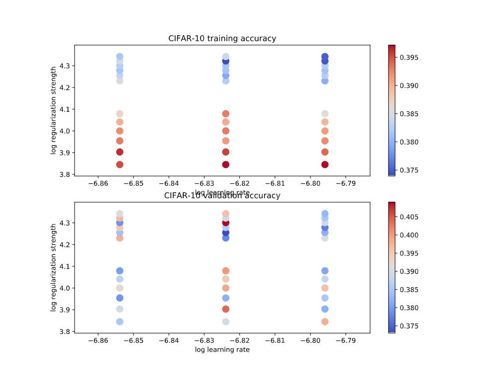
4. 计算多个学习率和正则化强度的准确率
实现思路:
- 两次循环计算即可
################################################################################
#  TODO :                                                                        #
# Write code that chooses the best hyperparameters by tuning on the validation #
# set. For each combination of hyperparameters, train a linear SVM on the      #
# training set, compute its accuracy on the training and validation sets, and  #
# store these numbers in the results dictionary. In addition, store the best   #
# validation accuracy in best_val and the LinearSVM object that achieves this  #
# accuracy in best_svm.                                                        #
#                                                                              #
# Hint: You should use a small value for num_iters as you develop your         #
# validation code so that the SVMs don't take much time to train; once you are #
# confident that your validation code works, you should rerun the validation   #
# code with a larger value for num_iters.                                      #
################################################################################
# *****START OF YOUR CODE (DO NOT DELETE/MODIFY THIS LINE)*****

svm  =   LinearSVM ()
for  learning_rate  in  learning_rates:
     for  reg  in  regularization_strengths:
        loss_hist  =  svm. train (X_train, y_train,  learning_rate = learning_rate,  reg = reg,
                       num_iters = 3000 ,  verbose = False )
        y_train_pred  =  svm. predict (X_train)
        train_accuracy  =  np. mean (y_train  ==  y_train_pred)
        y_val_pred  =  svm. predict (X_val)
        val_accuracy  = np. mean (y_val  ==  y_val_pred)
         if  val_accuracy  >  best_val:
            best_val  =  val_accuracy
            best_svm  =  svm
        results[(learning_rate,reg)] = (train_accuracy,val_accuracy)

# *****END OF YOUR CODE (DO NOT DELETE/MODIFY THIS LINE)*****
5. 多个学习率和正则化强度可视化结果


Summary
本次作业主要是SVM线性分类器的实现,由于对于python及numpy模块的不熟悉,导致作业完成得很吃力,希望能够加强掌握。
需要着重掌握numpy中数组的操作,灵活实现向量化运算。


